Tuần 7.2 Bayesian networks., AI Principle, CS221

Описание: playlist:    • CS221: Artificial Intelligence: Principles...  

github: https://github.com/hoanglong1712/Stan...

https://stanford-cs221.github.io/autu...
https://stanford-cs221.github.io/autu...

CS221: Artificial Intelligence: Principles and Techniques, Stanford

2025 05 09 02 06 36

Bayesian networks: overview
• In this module, I’ll introduce Bayesian networks, a new framework for modeling.
Course plan
Reflex
Search problems
Markov decision processes
Adversarial games
States
Constraint satisfaction problems
Markov networks
Bayesian networks
Variables Logic
Low-level High-level
Machine learning
CS221 2
• We have talked about two types of variable-based models.
• In constraint satisfaction problems, the objective is to find the maximum weight assignment given a factor graph.
• In Markov networks, we use the factor graph to define a joint probability distribution over assignments and compute marginal probabilities.
• Now we will present Bayesian networks, where we still define a probability distribution using a factor graph, but the factors have special
meaning.
• Bayesian networks were developed by Judea Pearl in the 1980s, and have evolved into the more general notion of generative modeling that
we see today.
Markov networks versus Bayesian networks
Both define a joint probability distribution over assignments
X1 X2 X3
t1
o1
t2
o2 o3
H1 H2 H3
E1 E2 E3
Markov networks Bayesian networks
arbitrary factors local conditional probabilities
set of preferences generative process
CS221 4
• Before defining Bayesian networks, it is helpful to compare and contrast Markov networks and Bayesian networks at a high-level.
• Both define a joint probability distribution over assignments, and in the end, both are backed by factor graphs.
• But the way each approaches modeling is different. In Markov networks, the factors can be arbitrary, so you should think about being able
to write down an arbitrary set of preferences and constraints and just throw them in. In the object tracking example, we slap on observation
and transition factors.
• Bayesian networks require the factors to be a bit more coordinated with each other. In particular, they should be local conditional probabilities,
which we’ll define in the next module.
• We should think about a Bayesian network as defining a generative process represented by a directed graph. In the object tracking example,
we think of an object as moving from position Hi−1 to position Hi and then yielding a noisy sensor reading Ei.
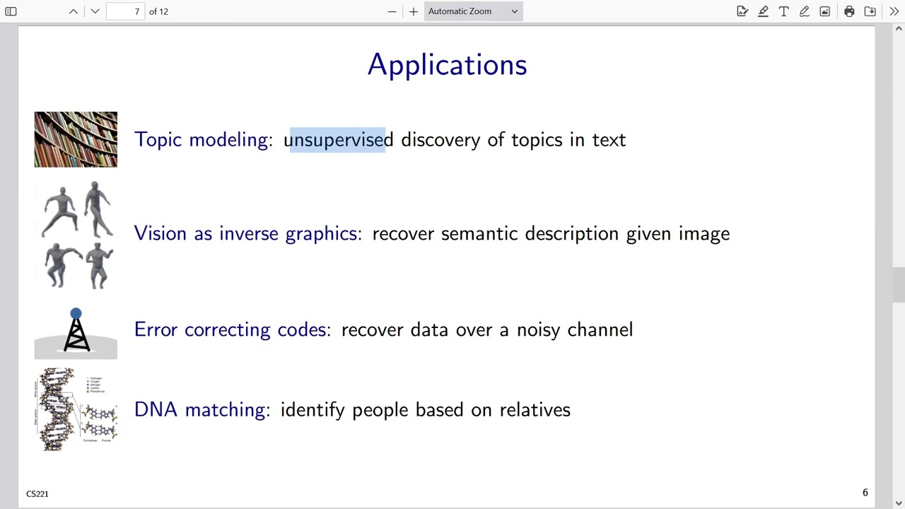
Applications
Topic modeling: unsupervised discovery of topics in text
Vision as inverse graphics: recover semantic description given image
Error correcting codes: recover data over a noisy channel
DNA matching: identify people based on relatives
CS221 6
• There are a huge number of applications of Bayesian networks, or more generally, generative models. One application is topic modeling, where
the goal is to discover the hidden structure in a large collection of documents. For example, Latent Dirichlet Allocation (LDA) posits that
each document can be described by a mixture of topics.
• Another application is a very different take on computer vision. Rather than modeling the bottom-up recognition using neural networks, which
is the dominant paradigm today, we can encode the laws of physics into a graphics engine which can generate an image given a semantic
description of an object. Computer vision is ”just” the inverse problem: given an image, recover the hidden semantic information (e.g.,
objects, poses, etc.). While the ”vision as inverse graphics” perspective hasn’t been scaled up beyond restricted environemnts, the idea seems
tantalizing.
• Switching gears, in a wireless or Ethernet network, nodes must send messages (a sequence of bits) to each other, but these bits can get
corrupted along the way. The idea behind error correcting codes (Low-Density Parity Codes in particular) is that the sender also sends a set
of random parity checks on the data bits. The receiver obtains a noisy version of the data and parity bits. A Bayesian network can then be
defined to relate the original bits to the noisy bits, and the receiver can use inference (usually loopy belief propagation) to recover the original
bits.
• The final application that we’ll discuss is DNA matching. For example, Bonaparte is a software tool developed in the Netherlands that uses
Bayesian networks to match DNA based on a candidate’s family members. There are two use cases, the first one is controversial and the
second one is grim. The first use case is in forensics: given DNA found at a crime site, even if the suspect’s DNA is not in the database, one
can match it against the family members of a suspect, where the Bayesian