MECH 516 Lecture# 10 .Source Panel Method with Matlab Code

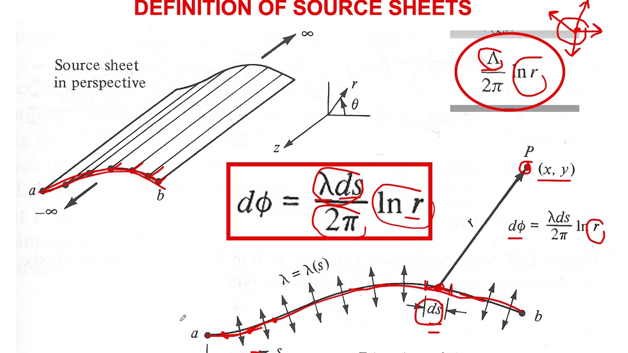
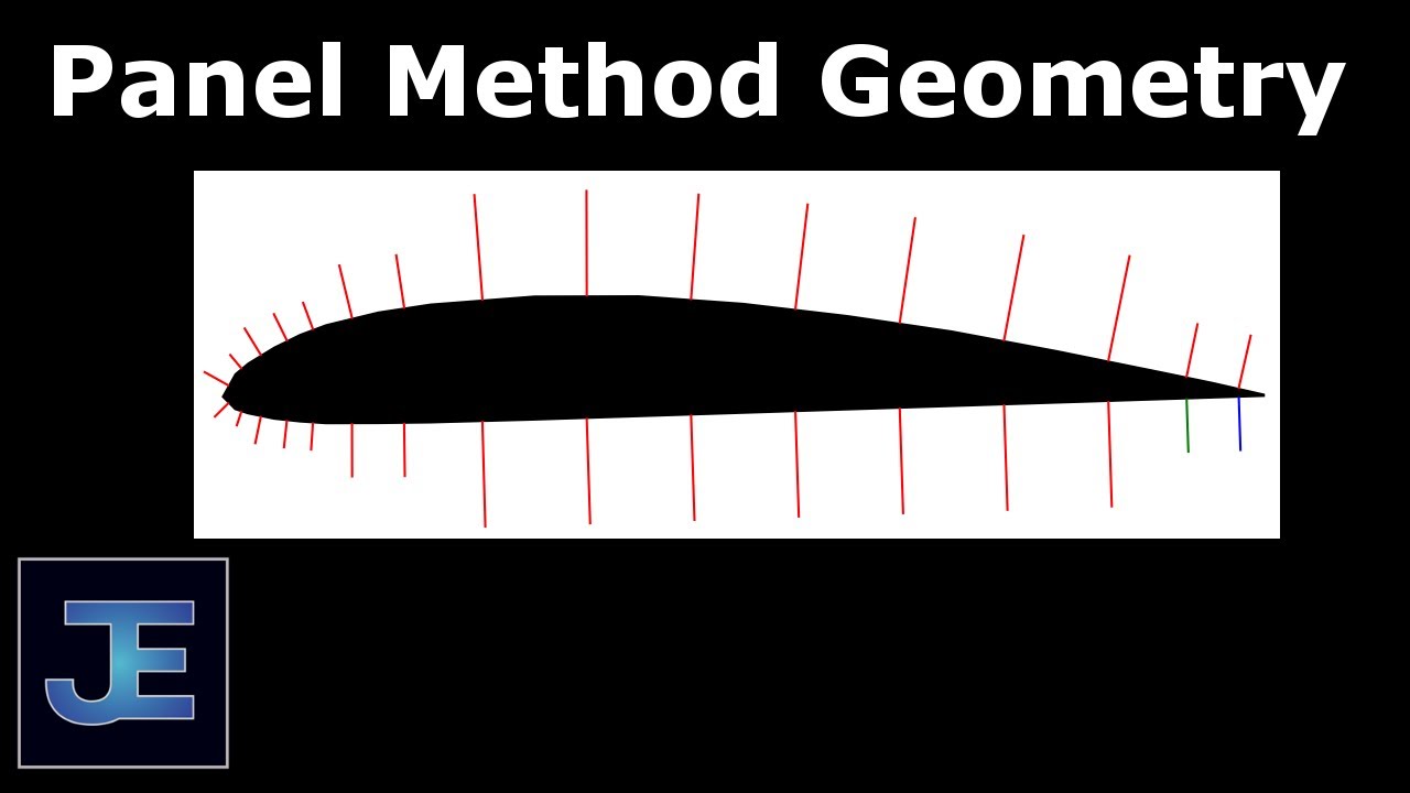
Описание: Source panel method with application to circular cylinder flow

Note: In two lines in the code below replace .lt. with the angled bracket symbol because YT doesn't accept angled brackets

CODE:
close all
clear
clc
V0=1; % free stream V_infinity
alfa=0*pi/180; % freestream angle with the horziontal
k=0;

% Defining body geometry: circle

R=1.0;
step=-22.50/2;
for thd=180 + step/2:step:-180 -step/2
k=k+1; % panel number k
th=thd*pi/180;
x(k)=R*cos(th);
y(k)=R*sin(th);
end
% just for plotting
x(k+1)=R*cos(th+step*pi/180); % just for plotting to close the body
y(k+1)=R*sin(th+step*pi/180); % just for plotting to close the body

% velocity at control point
V(k)=0;
% Defining control points for panels
for i=1:1:k
% panel edges
X(i)=x(i);
Y(i)=y(i);
% control points (xcp,ycp)
xcp(i)=( x(i) + x (i+1) )/2;
ycp(i)=( y(i) + y (i+1) )/2;
TH(i)=atan2(ycp(i),xcp(i));
% length of panel
lngp(i)=sqrt(( x(i) - x (i+1))^2 + (y(i) - y (i+1))^2);
% slope of panel (angle with the horizontal, from LE)
phi(i)= atan2(( y(i+1) - y (i) ),( x(i+1) - x (i) ));
end
X(i+1)=x(i+1);
Y(i+1)=y(i+1);
%X(i+2)=x(1);
%Y(i+2)=y(1);
%xcp(i+1)=( x(i+1) + x (i+2) )/2;
%ycp(i+1)=( y(i+1) + y (i+2) )/2;
%TH(i+1)=atan2(ycp(i+1),xcp(i+1));
%lngp(i+1)=sqrt(( x(i+2) - x (i+1))^2 + (y(i+2) - y (i+1))^2);
%phi(i+1)= atan(( y(i+2) - y (i+1) )/( x(i+2) - x (i+1) ));

figure
plot(x,y)
axis([-4 4 -4 4]*.4)
axis square
text(xcp*1.1,ycp*1.1,num2str(round(phi'*1800/pi)/10))
hold on
plot(xcp,ycp,'r.')
xlabel('x','FontWeight','bold');ylabel('y','FontWeight','bold');
title('labels: angle: \phi','FontWeight','bold')

figure
plot(x,y)
axis([-4 4 -4 4]*.4)
axis square
text(xcp*1.1,ycp*1.1,num2str(round(TH'*1800/pi)/10))
hold on
plot(xcp,ycp,'r.')
xlabel('x','FontWeight','bold');ylabel('y','FontWeight','bold');
title('labels: angle: \theta','FontWeight','bold')
%beta: angle between panel normal and the freestream
beta= phi - alfa + pi/2;
% Setting up the linear system of equations (source panels)
for i=1:1:k
for j=1:1:k
if j~=i
A=-(xcp(i)-X(j))*cos(phi(j))...
-(ycp(i)-Y(j))*sin(phi(j));
B=(xcp(i)-X(j))^2 + (ycp(i)-Y(j))^2;
C=sin(phi(i)-phi(j));
D=(ycp(i)-Y(j))*cos(phi(i))...
-(xcp(i)-X(j))*sin(phi(i));
S(j)=sqrt( (X(j+1)-X(j))^2 ...
(Y(j+1)-Y(j))^2 );
E=sqrt(B-A^2);
I(i,j)=C/2*log( (S(j)^2+ 2*A*S(j)+B)/B )...
+(D-A*C)/E* (atan2((S(j)+A),E)...
-atan2(A,E));
a(i,j)=1/(2*pi)*I(i,j);
% I(i,j)= Integral[(d/dn_i(ln r_i,j))]ds
if i==4 & j==2
[A B C D S(j) E];
end
elseif i==j
a(i,j)=1/2;
end
end
b(i)=V0*cos(beta(i));
end
% solving the linear system of equations for lambda
% a * lambda + b = 0
lambda=linsolve(a,-b');
dum=lambda/(2*pi*V0);
figure
plot(x,y)
hold on
plot(xcp,ycp,'r.')
text(xcp*1.1,ycp*1.1,num2str(round(dum*1e4)/1e4))
xlabel('x','FontWeight','bold');ylabel('y','FontWeight','bold');
title('labels: \lambda / (2\pi V_{\infty})','FontWeight','bold')
axis([-4 4 -4 4]*.4)
axis square
%%%% PART 2 --- Evaluating the velocity at the control pts
for i=1:1:k
for j=1:1:k
if i~=j
A=-(xcp(i)-X(j))*cos(phi(j))...
-(ycp(i)-Y(j))*sin(phi(j));
B=(xcp(i)-X(j))^2 + (ycp(i)-Y(j))^2;
C=sin(phi(i)-phi(j));
D=(ycp(i)-Y(j))*cos(phi(i))...
-(xcp(i)-X(j))*sin(phi(i));
S(j)=sqrt( (X(j+1)-X(j))^2 ...
(Y(j+1)-Y(j))^2 );
E=sqrt(B-A^2);
J(i,j)=((D-A*C)/(2*E))*log( (S(j)^2+ 2*A*S(j)+B)/B )...
C * (atan2((S(j)+A),E)- atan2(A,E));
a(i,j)=1/(2*pi)*I(i,j);
% the velocity at the control point
V(i)=V(i) + lambda(j)/(2*pi)*J(i,j);
end
end

V(i)= V(i) + V0*sin(beta(i));
cp(i)=1-(V(i)/V0)^2;
end

for i=1:1:size(phi,2)
for j=i+1:1:size(phi,2)
% YouTube Error: lt: replace with less than
if phi(j) .lt. phi(i)
dum1=phi(i);
phi(i)=phi(j);
phi(j)=dum1;
dum1=TH(i);
TH(i)=TH(j);
TH(j)=dum1;
dum1=cp(i);
cp(i)=cp(j);
cp(j)=dum1;
end
end
end

figure, plot(phi*180/pi,cp,'x-')
xlabel('\phi','FontWeight','bold');ylabel('C_p','FontWeight','bold');
title('C_p','FontWeight','bold')

for i=1:1:size(TH,2)
for j=i+1:1:size(TH,2)
% YouTube Error: lt: replace with less than
if TH(j) .lt. TH(i)
dum1=TH(i);
TH(i)=TH(j);
TH(j)=dum1;
dum1=cp(i);
cp(i)=cp(j);
cp(j)=dum1;
end
end
end
figure, plot(TH*180/pi,cp,'x-')
xlabel('\theta','FontWeight','bold');
ylabel('C_p','FontWeight','bold'); %title('C_p')