Exp22_Excel_Ch07_CumulativeAssessment_Variation_Shipping | Exp22 Excel Ch07 CumulativeAssessment

Описание: Exp22_Excel_Ch07_CumulativeAssessment_Variation_Shipping | Exp22 Excel Ch07 CumulativeAssessment


#Exp22_Excel_Ch07_CumulativeAssessment_Variation_Shipping#Excel_Ch07_CumulativeAssessment_Variation_Shipping#Excel_Ch07_CumulativeAssessment_Variation#Exp22_Excel_Ch07_Cumulative
#Ch07_CumulativeAssessment_Variation#CumulativeAssessment_Variation_Shipping#CumulativeAssessment_Variation#Variation_Shipping#Variation_Shipping.xlsx#Exp22_Excel_Ch07_Cumulativ#Excel_Ch07_CumulativeAssessment#Excel_Ch07#Ch07_CumulativeAssessment#exp22_excel_ch07_cumulativeassessment_shipping#shipping









Contact
WhatsApp 1: +92 3227697093
WhatsApp 2: +92 3255683413
Email:: : [email protected]
Direct WhatsApp link
Link : https://wa.link/d27yzv








In cell D7, insert the appropriate date function to calculate the number of days between the Date Arrived and Date Ordered. Copy the function to the range D8:D35.

Hint: Formula is =DAYS(Date Arrived, Date Ordered) 5
3 You want to display the weekday for the arrival dates.

In cell E7, insert the WEEKDAY function to identify an integer representing the weekday of the Date Arrived. Copy the function to the range E8:E35.
Hint: Formula is =WEEKDAY(Date Arrived). 4
4 You need to format the WEEKDAY function results with a custom number format.

Select the range E7:E35, apply the custom number format dddd, and apply center horizontal alignment. 2
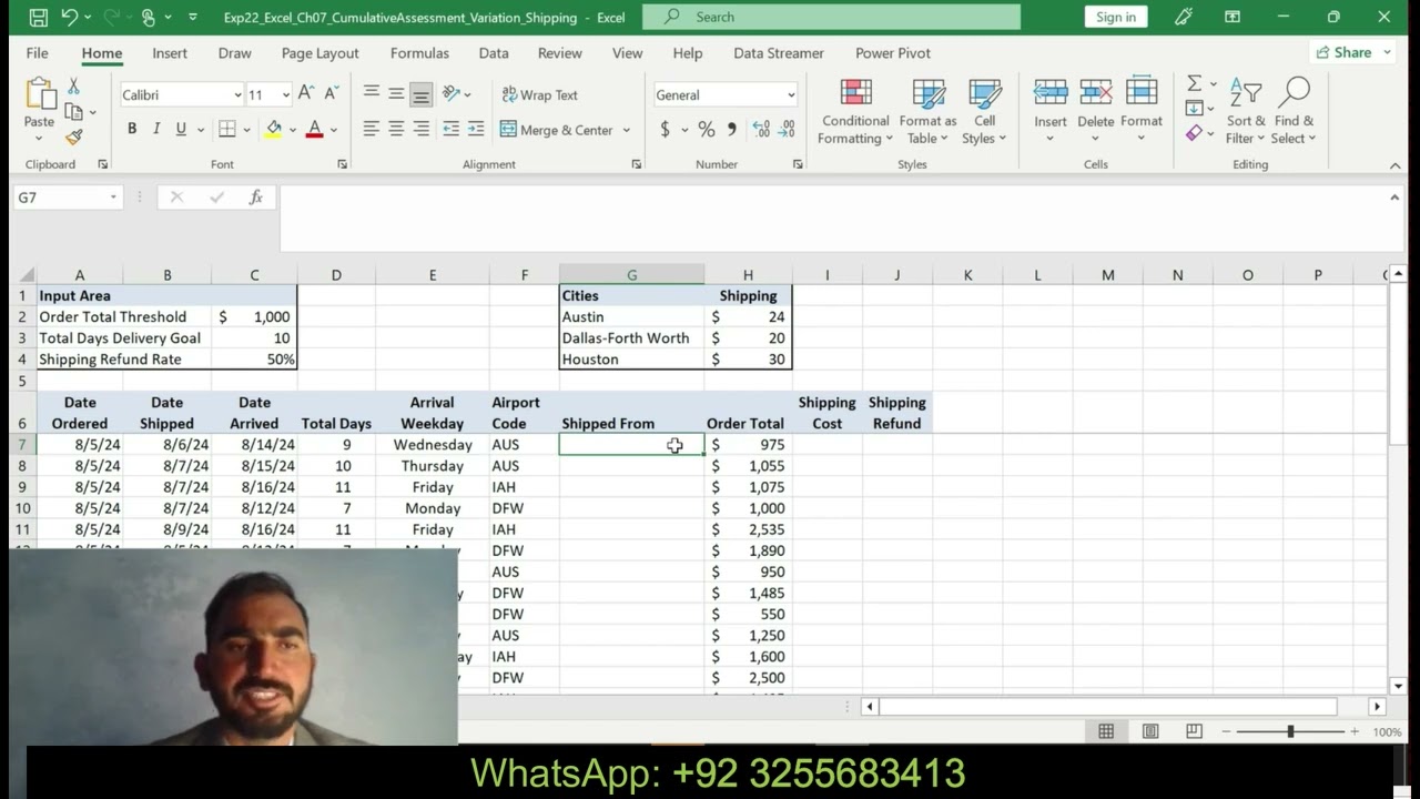
5 Next, you want to display the city names that correspond with the city airport codes.

In cell G7, insert the SWITCH function to evaluate the airport code in cell E7. Include mixed cell references to the city names in the range G2:G4. Use the airport codes as text for the Value arguments: AUS for Austin, DFW for Dallas-Fort Worth, and IAH for Houston. Copy the function to the range G8:G35.

Hint: Formula is =SWITCH(Airport Code, AUS, cell reference to Austin, DFW, cell reference to Dallas-Fort Worth, IAH, cell reference to Houson) 5
6 Now you want to display the standard shipping costs by city.

In cell I7, insert the IFS function to identify the shipping cost based on the airport code and the applicable shipping rates in the range H2:H4. Enter the airport codes in this sequence: AU