EX2024-IndependentProject-3-4 | Classic Gardens and Landscapes (CGL) | ClassicGardens-03

Описание: Steps to complete This Project
Mark the steps as checked when you complete them.
1. Open the ClassicGardens-03 start file. If the workbook opens in Protected View, click the Enable Editing button so you can modify it. The file will be renamed automatically to include your name. Change the project file name if directed to do so by your instructor, and save it.
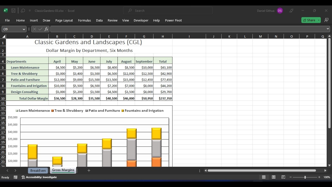
2. Use the Recommended Charts command to create a Stacked Column chart object for cells A4:G9 on theGross Margins sheet.
3. Move the chart object so that its top-left corner is at cell A12. Size the chart to reach cell H30.
4. Apply a 1 pt Black, Text 1 (second column) outline to the chart area.
5. Select each data series and apply a Circle bevel.
6. Display the primary minor horizontal axis gridlines. Format the major value axis gridlines with a Black, Text 1outline color. Do not change the color for the minor gridlines.
7. Resize the data range to remove the Design Consulting data series from the chart (Figure 3-85 ).
8. Delete the title and format the legend.
a. Delete the chart title object.
b. Select the legend and position it at the top of the chart area.
c. Format the legend font size to 12 [Home tab].
d. Click the Patio and Furniture legend entry and change its fill color to Light Gray Background 2, Darker 25%.
e. Change the Lawn Maintenance legend entry fill color to Green, Accent 6, Lighter 80%.
f. Select the legend and apply bold.
9. Format the plot area.
a. Select the plot area and apply a ¼ pt Black, Text 1 outline.
b. Apply an Offset: Bottom Right shadow to the plot area.
c. Select cell A1.
10. Review break-even formulas and build the data source for a line chart.
a. Click the BreakEven sheet tab.
b. Select cell B8. The margin (profit) per unit is calculated by subtracting the variable cost (B6) from the sales price (B5).
c. Select cell B10. The formula divides the fixed cost (B7) by the sales price minus the variable cost (B5-B6). That part of the formula is nested within a ROUND function to show no decimal places.
d. Review the references and formulas in row 15.
e. Copy the formulas in row 15 to reach row 24.
f. Select cell B5 and type 200. Verify that at this price, the break-even point is 200 units. This is the level at which all costs are covered and there is no profit.
11. Create a line chart.
a. Select cells B14:C24 and E14:F24, four columns in the table.
b. Create a 2-D Line chart with markers.
c. Position the chart object to start at cell A26 and to reach cell H45.
12. Edit the source data.
a. Click the Select Data button [Chart Design tab, Data group]. The horizontal axis labels are numbers 1 through 10 in the chart.
b. Click the Horizontal (Category) axis labels box.
c. Select cells B15:B24 for the Axis label range (Figure 3-86). The Select Data Source dialog box is still open.
d. Click the # Sold label in the Legend entries (Series) list and click the Delete button (the - sign). These values are not category labels and should not be plotted as a line (Figure 3-87).
e. Click OK.
13. Edit the chart title to display Break Even for Planter Sales. Select the label and make it Black, Text 1 andbold.
14. Display and format chart elements.
a. Use the Chart Elements drop-down list to select the legend and position it at the top.
b. Display the primary major horizontal and vertical gridlines.
c. Format both vertical and horizontal gridlines with Black, Text 1, Lighter 50% for the Shape Outline.
d. Apply a 1 pt Black, Text 1 outline for the chart area.
e. Apply an Offset: Bottom Right shadow effect to the plot area.
15. Change the sales price to $225 (cell B5).
16. Insert and format a shape in a chart.
a. Select the chart object, and find and click the Oval shape in the Basic Shapes group [Format tab, Insert Shapes group].
b. Draw an oval around the break even point in the chart as shown in Figure 3-88 . At break even, sales and total costs are equal.

c. Select the oval shape and change its Shape Fill [Shape Format tab, Shape Styles group] to No Fill.
d. Change its Shape Outline [Shape Format tab, Shape Styles group] to Red in the Standard Colors group.
e. Select the Fixed Cost line in the chart and change its color to Black, Text 1. Change its marker color and marker border to Black, Text 1.
17. Complete worksheet formatting.
a. Select cells A1:A3 and change the font size to 16.
b. Select cells A1:H3 and center the cells across the selection.
c. Apply a bottom border to cells A3:H3.
d. Select cell A1.
e. Set the page for landscape orientation, center the page horizontally, and scale it to fit one page.
18. Save and close the workbook (Figure 3-89).