Суммирование дубликатов в Excel — Советы и рекомендации по Excel

Описание: Узнайте, как суммировать дубликаты в Excel.

Для суммирования дубликатов в Excel можно использовать функцию «Удалить дубликаты» на вкладке «Данные», которая позволяет выбрать столбцы с дубликатами и удалить лишние записи, оставив только уникальные. Чтобы изолировать дубликаты, примените условное форматирование или используйте встроенные в Excel правила выделения ячеек, чтобы выделить дублирующиеся значения в наборе данных. Чтобы сгруппировать дубликаты, можно создать сводную таблицу с данными, а затем использовать функцию «Группировка» для объединения дубликатов. При работе с дубликатами в нескольких списках рассмотрите возможность использования функции «Консолидировать» или формул «ВПР» или «ИНДЕКС-ПОИСКПОЗ» для поиска и агрегации совпадающих значений. Для суммирования схожих данных в Excel незаменимы сводные таблицы и функции группировки. Для суммирования значений с одинаковыми именами можно использовать функцию «СУММЕСЛИ» или «СУММЕСЛИМН». Работая в Google Таблицах, вы можете использовать меню «Данные» для группировки дубликатов или совпадающих значений в наборе данных. Чтобы объединить дубликаты в Excel без потери данных, используйте функцию «Консолидация» или напишите собственные скрипты VBA, которые интеллектуально объединяют дубликаты записей, сохраняя важную информацию и устраняя избыточность.

Вот шаги, описанные в видео.

Определить дубликаты
1) Щёлкните правой кнопкой мыши
2) Найдите «дубликат»
3) Выберите «Повторяющееся значение»

Определить дубликаты (длинный способ)
1) Выберите «Пользователи 1» и «Пользователи 2»
2) Главная ~ Стиль ~ Условное форматирование
3) Правила выделения ячеек ~ Повторяющиеся значения...
4) ОК

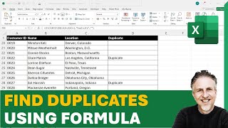
Объединить список дубликатов
=ФИЛЬТР(A2:A27;СЧЁТЕСЛИ(B2:B33;A2:A27))

Вот как выглядит формула:

1) ФИЛЬТР(A2:A27; ... ): Это функция ФИЛЬТР, которая возвращает массив значений, удовлетворяющих заданному условию. В данном случае она фильтрует значения из диапазона A2:A27.
2) СЧЁТЕСЛИ(B2:B33; A2:A27): Эта часть формулы вычисляет, сколько раз каждое значение из диапазона A2:A27 встречается в диапазоне B2:B33.
B2:B33 — это диапазон, в котором проверяется наличие значений из диапазона A2:A27.
A2:A27 — это диапазон значений, который нужно отфильтровать.
3) СЧЁТЕСЛИ подсчитывает, сколько раз каждое значение из диапазона A2:A27 встречается в диапазоне B2:B33.
4) СЧЁТЕСЛИ возвращает массив счётчиков, где каждый счётчик соответствует значению из диапазона A2:A27.
5) Функция ФИЛЬТР использует этот массив счётчиков в качестве условия. Она фильтрует значения из диапазона A2:A27, полагая, что счётчик больше нуля, что означает, что значение из диапазона A2:A27 встречается хотя бы один раз в диапазоне B2:B33.

Таким образом, результатом этой формулы является массив значений из диапазона A2:A27, которые также присутствуют в диапазоне B2:B33. Любое значение из диапазона A2:A27, которое отсутствует в диапазоне B2:B33, не будет включено в отфильтрованный список.

🔗🔗 ССЫЛКИ НА ПОХОЖИЕ ВИДЕО 🔗🔗
Как сравнить два списка и найти пропущенные значения БЕЗ ФОРМУЛ в Excel — Советы и рекомендации по Excel
   • How to compare two lists to find missing v...  

Сравнение двух списков и поиск пропущенных значений с помощью функции XLOOKUP в Excel — Советы и рекомендации по Excel
   • Compare two lists to find missing values u...  

Сравнение двух списков и поиск пропущенных значений с помощью функции VLOOKUP в Excel — Советы и рекомендации по Excel
   • Compare two lists to find missing values u...  

Как сравнить два списка в Excel с помощью условного форматирования — Советы и рекомендации по Excel Хитрости
   • How to compare two lists in Excel using Co...  

Как сравнить два списка в Excel и найти пропущенные значения — Советы и хитрости по Excel
   • How to compare two lists to find missing v...  

Советы и хитрости по Excel — Сравнение двух списков в Excel
   • Excel Tips and Tricks - Compare Two Lists ...  

Суммирование дубликатов в Excel — Советы и хитрости по Excel
   • Summarize Duplicates in Excel - Excel Tips...  

Быстрое нахождение различий в Excel: сравнение двух списков — Советы и хитрости по Excel Хитрости
   • Find difference quickly in Excel Comparing...  

#совет #excel #microsoft #shorts #shortvideo #shortsvideo #howto #как #google